Equilibrating a box of acetonitrile with MD

Goals

In this tutorial we learn how to perform a thermal equilibration of a box of acetonitrile molecules using ASE. We will:

• build a coarse-grained CH₃–C≡N triatomic model.

• set up a periodic box at the experimental density (298 K).

• apply rigid-molecule constraints.

• use the ACN force field.

• equilibrate with Langevin dynamics.

• scale small box of 27 molecules to 216 molecules.

ACN model

The acetonitrile force field implemented in ASE (ase.calculators.acn) is an interaction potential between three-site linear molecules. The atoms of the methyl group are treated as a single site centered on the methyl carbon (hydrogens are not explicit). Therefore:

• assign the methyl mass to the outer carbon (m_me),

• use the atomic sequence Me–C–N repeated for all molecules,

• keep molecules rigid during MD with FixLinearTriatomic.

import matplotlib.pyplot as plt
import numpy as np

import ase.units as units
from ase import Atoms
from ase.calculators.acn import ACN, m_me, r_cn, r_mec
from ase.constraints import FixLinearTriatomic
from ase.io import Trajectory
from ase.md import Langevin
from ase.visualize.plot import plot_atoms

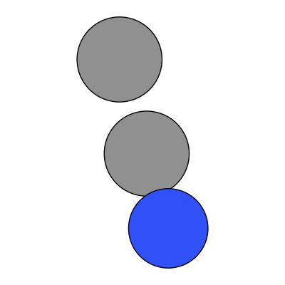
Step 1: Molecule

Build one CH3–C≡N as a linear triatomic “C–C–N”. The first carbon is the methyl site; we assign it the CH3 mass. Rotate slightly to avoid perfect alignment with the cell axes.

pos = [[0, 0, -r_mec], [0, 0, 0], [0, 0, r_cn]]
atoms = Atoms('CCN', positions=pos)
atoms.rotate(30, 'x')

masses = atoms.get_masses()
masses[0] = m_me
atoms.set_masses(masses)

mol = atoms.copy()
mol.set_pbc(False)
mol.set_cell([20, 20, 20])
mol.center()

fig, ax = plt.subplots(figsize=(4, 4))
plot_atoms(
    mol,
    ax=ax,
    rotation='30x,30y,0z',
    show_unit_cell=0,
    radii=0.75,
)
ax.set_axis_off()
plt.tight_layout()
plt.show()

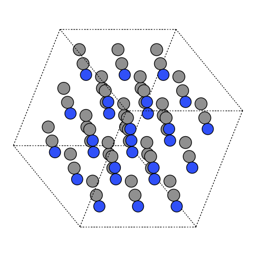
Step 2: Set up small box of 27-molecules

Match density 0.776 g/cm^3 at 298 K. Compute cubic box length L from mass and density. Build 3×3×3 supercell and enable PBC.

density = 0.776 / 1e24  # g / Å^3
L = ((masses.sum() / units.mol) / density) ** (1 / 3.0)

atoms.set_cell((L, L, L))
atoms.center()
atoms = atoms.repeat((3, 3, 3))
atoms.set_pbc(True)

box27 = atoms.copy()
fig, ax = plt.subplots(figsize=(5, 5))
plot_atoms(
    box27,
    ax=ax,
    rotation='35x,35y,0z',
    show_unit_cell=2,
    radii=0.75,
)
ax.set_axis_off()
plt.tight_layout()
plt.show()

Step 3: Set constraints

Keep each “C–C–N” rigid during MD using FixLinearTriatomic.

nm = 27
triples = [(3 * i, 3 * i + 1, 3 * i + 2) for i in range(nm)]
atoms.constraints = FixLinearTriatomic(triples=triples)

Step 4: MD run for 27-molecules system

Assign ACN with cutoff = half the smallest box edge. Langevin MD at 300 K, 2 fs timestep. Save a frame every step.

Note

This example uses a relatively large timestep to demonstrate the usage of the code. In general, a smaller timestep should be used for this molecular dynamics simulation. Generally, the timestep depends on the chemical system, its constraints and is in the order of 0.5-2~fs.

atoms.calc = ACN(rc=np.min(np.diag(atoms.cell)) / 2)

tag = 'acn_27mol_300K'
md = Langevin(
    atoms,
    2 * units.fs,
    temperature_K=300,
    friction=0.01,
    logfile=tag + '.log',
)
traj = Trajectory(tag + '.traj', 'w', atoms)
md.attach(traj.write, interval=50)  # writing the structure every 100 fs
md.run(10)  # 10 timestseps @ 2 fs = 0.02 ps

True

Step 4: Monitoring a MD simulation

Tracking different properties such as the temperature of a system makes sense to monitor the behavior of a system and insure correct physics.

times_ps, epots, ekins, etots, temps = [], [], [], [], []
sample_interval = 10  # sample every 10 MD steps for lighter plots


def sample():
    # Time in ps (same as MDLogger: dyn.get_time() / (1000 * units.fs))
    t_ps = md.get_time() / (1000.0 * units.fs)
    ep = atoms.get_potential_energy()  # eV total
    ek = atoms.get_kinetic_energy()  # eV total
    T = atoms.get_temperature()  # K
    times_ps.append(t_ps)
    epots.append(ep)
    ekins.append(ek)
    etots.append(ep + ek)
    temps.append(T)


# initial sample at t=0
sample()
md.attach(sample, interval=sample_interval)
md.run(1500)  # 1500 timesteps @ 2 fs = 3 ps

True

Plot Instantaneous temperature vs time. Does the system equilibrated well? What is the average temperature? Should we run longer simulations?

fig, ax = plt.subplots(figsize=(6, 4))
# line at 300 K for comparison
ax.axhline(300, color='black', linestyle='--')
ax.plot(times_ps, temps, label='T (K)')
ax.set_xlabel('Time (ps)')
ax.set_ylabel('Temperature (K)')
ax.legend(loc='best')
ax.grid(True, linewidth=0.5, alpha=0.5)
plt.tight_layout()
plt.show()

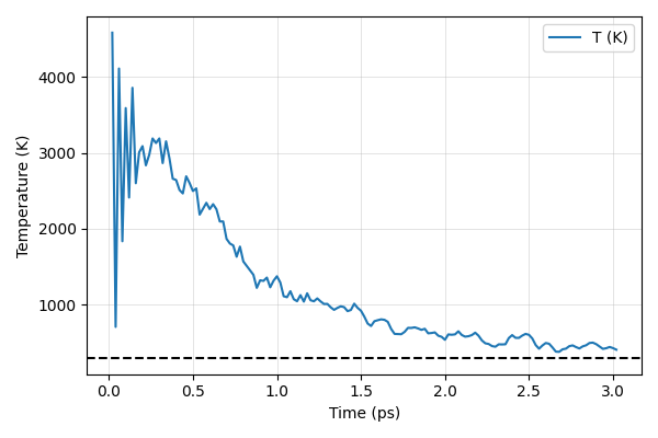
Hint: How does the temperature of the atoms align with the black dashed line at 300 K? Try running for 5 ps and 10 ps, is the system equilibrated then?

Step 6: Scale system size to 216 molecules

Repeat 2×2×2 to reach 216 molecules. Reapply constraints and update the ACN cutoff for the new cell.

atoms.set_constraint()
atoms = atoms.repeat((2, 2, 2))

nm = 216
triples = [(3 * i, 3 * i + 1, 3 * i + 2) for i in range(nm)]
atoms.constraints = FixLinearTriatomic(triples=triples)

atoms.calc = ACN(rc=np.min(np.diag(atoms.cell)) / 2)

Step 7: MD run for 216-molecules system

tag = 'acn_216mol_300K'
md = Langevin(
    atoms,
    2 * units.fs,
    temperature_K=300,
    friction=0.01,
    logfile=tag + '.log',
)
traj = Trajectory(tag + '.traj', 'w', atoms)
md.attach(traj.write, interval=50)

times_ps, epots, ekins, etots, temps = [], [], [], [], []
sample_interval = 10  # sample every 10 MD steps for lighter plots

# initial sample at t=0
sample()
md.attach(sample, interval=sample_interval)
md.run(10)  # 10 timesteps @ 2 fs = 0.02 ps

True

This simulation is only run very briefly to show how to scale a simulation. Try running the simulation longer and plot the temperature and other properties. Does this size take longer to equilibrate?

Next steps

• View trajectories:

  ase gui acn_27mol_300K.traj
  
  ase gui acn_216mol_300K.traj
  

• Plot other thermodynamic quantities (p.e., k.e., and total energy).